\(~\)
Background
Both the CDC and the WHO consider obesity an epidemic, a “major contributor to the global burden of chronic disease and disability.”1 BMI is the most common measure of obesity, and is the general standard by which overweight and obesity are classified. It’s important to acknowledge, though, that BMI is a proxy for the thing that ostensibly concerns us: adiposity, i.e., body fat. The CDC make note on their website that BMI is a screening tool, not a diagnostic, and thus requires follow-up testing for confirmation and further consideration of individual health status and risks.2
BMI is a source of contention in its own right; many researchers, practitioners, and concerned parties worry that it misclassifies many individuals, and worse, that the cut-offs are rather arbitrary. Defenders of BMI point to its utility as an initial screening tool, and a pretty successful one at that.
The controversy does not end there. Despite the consistent association of adiposity and a variety of health risks, many researchers have observed improved survival among ill or elderly cohorts with BMI statuses above the range traditionally deemed healthy, meaning those considered overweight and/or obese. This is pretty surprising to a lot of people: greater adiposity is associated with increased risk of a variety of disease states, and yet overweight status seems to be protective against death, and even some level of obesity does not confer any disadvantage compared to normal weight people.
This 2013 meta-analysis by Flegal et al. is perhaps the most famous (or infamous) paper to show these counterintuitive findings on a large scale, though the term had been around for at least decade before it was published. A 2016 meta-analysis by the Global BMI Mortality Collaboration can be considered something of a response to Flegal’s paper. It contains more studies from more countries with more participant data, and uses a some different methods to limit reverse causality. The appropriateness of these methods is naturally the source of much debate all on its own, but a discussion of this is beyond the scope of our current investigation here.
There are many many more papers I can cite that explore, support, criticize, or discuss the obesity paradox. The particular thing, however, that I’d like to draw attention to is that they almost all use BMI as a measure of obesity status. Indeed, BMI is the primary measure by which our epidemiological obesity research is conducted, and consequently by which our conclusions are made. Despite the known lack of resolution at the individual level, BMI seems to be taken for granted as an appropriate and informative tool in these large-scale analyses. Subsequent debates about the role of body fat in health and mortality rely on conclusions which assume that such results accurately reflect body compostion in the first place.
But do they? After all, body fat is only one source of weight—we also have bones, organs, and muscle tissue. It’s not likely that bone and organ mass would lead to large differences in body mass at any given height when dealing with large populations, but muscle tissue sure can. In fact, muscle tissue is already a known determinant of health status, particularly in the elderly. Sarcopenia is a potent cause of concern in advancing age. However, given increasingly sedentary lifestyles, muscle tissue status might a growing concern at younger ages. At the very least, it seems worth investigating, especially since body fat has commanded the spotlight so exclusively for so long.
\(~\)
The Question
The simple question that a lot of researchers spend a lot of time on trying to resolve is, what is the cause of the apparent obesity paradox? Alternatively, is there a paradox in need of resolving?
We won’t be able to definitively answer either question in one blog post, but we can definitely gain some insight into possible reasons for why these discrepancies exist. I think it makes sense to check our tools when something doesn’t seem quite right, so it’ll help us to get a better sense of how BMI “behaves.”
I’ve also had a pet theory for a while that the status of lean tissue, and muscle mass in particular, might help explain common inconsistencies. The bulk of the literature in this area concerns BMI and body fat; in comparison, not much mention is made of muscle mass. So one component of our investigation will concern the particularities of muscle tissue status within the official BMI categories.
The ultimate aim of this analysis will be to more carefully assess the construct validity of BMI itself. Construct validity refers to the ability of the particular form of measurement to accurately represent the actual construct of interest. For example, does IQ adequately capture the not directly observable abstraction we call intelligence? Thankfully, our “construct” here is body fat, which is quite observable, so we don’t have to worry so much about the characteristics of theory here. All we need is a more direct measure of body fat, which is not all that hard to find…
\(~\)
Sourcing the Data
We’ll use data from the National Health and Nutrition Examination Survey (NHANES)3, a yearly survey of population health status and disease prevalence from a representative sample of 5000 participants. NHANES is a flagship program of the NAtional Center for Health Statistics (NCHS), which is part of the CDC.
Our data set will cover the year 1999-2006, because these are the years for which dual X-ray absorbtriometry (DXA) scans were included in the health examinations. DXA scans are considered a gold standard measurement tool for body composition. Other years use other tools, such as bioelectrical impedance, but I want to keep the data as consistent and reliable as possible.
NHANES includes a wealth of data including hundreds variables across numerous examinations and questionnaires. We’re interested of course in body composition and certain demographic characteristics. Another benefit of NHANES data is that the CDC has linked these data sets to participant mortality data up to the year 20154 (with subsequent years incoming), so we can choose to investigate associations with mortality if we want to perform a bit of inference in the future. All in all it’s an extremely rich source of population data.
\(~\)
The Data
\(~\)
Libraries
These are the packages we need to run all of our code.
library(tidyverse)
library(foreign)
library(parsnip)
\(~\)
Importing the Data
I downloaded the files for each year that NHANES inlcuded DXA scans and for which there is linked mortality data. This included demographics, body measures, and dual-energy x-ray absorptiometry data from survey years 1999-2000, 2001-2002, 2003-2004, and 2005-2006. The data files are in two year groups because, though surveys are conducted yearly, data are released in two year batches for the purpose of larger sample sizes with more precise inferences.
\(~\)
Cleaning the Data
The bulk of what we need to do is trim and combine the data sets, which also requires some alterations so that the joins work. We’ll also rename the variables to make them more understandable.
nrow(dat)## [1] 29026There are just over 29,000 observations, but missingness has not yet been accounted for.
| x | |
|---|---|
| id | 0 |
| l_arm | 1767 |
| r_arm | 1767 |
| l_leg | 1767 |
| r_leg | 1767 |
| perc_fat | 1767 |
| weight | 568 |
| height | 455 |
| bmi | 709 |
| gender | 0 |
| age | 0 |
| age_m | 468 |
| mortstat | 8671 |
Several columns contain missing values, but by filtering three of the most important variables we can drastically reduce missingness in the data set. I’ve decided to allow for some missing age-in-months observations since there are relatively few missing in total. The other variables are too important to allow missing values for.
knitr::kable(
  colSums(is.na(dat))
)| x | |
|---|---|
| id | 0 |
| l_arm | 0 |
| r_arm | 0 |
| l_leg | 0 |
| r_leg | 0 |
| perc_fat | 0 |
| weight | 0 |
| height | 0 |
| bmi | 0 |
| gender | 0 |
| age | 0 |
| age_m | 390 |
| mortstat | 0 |
nrow(dat)## [1] 18536About 10,500 participants have been lost after removing NAs, mostly due to missing mortality data, but the data set is still quite large. Unfortunately, the missing mortality data cannot be imputed safely because we cannot make any safe assumptions about the various reasons why such data might be missing in the first place.
\(~\)
Adding New Variables
We’ll add the official BMI designation for each observation.
# Create BMI categories and add new variable
bmi_levels = c("Underweight", "Healthy", "Overweight", "Obese")

dat <- dat %>%
  mutate(bmi_status = case_when(bmi >= 30 ~ "Obese",
                         bmi < 30 & bmi >= 25 ~ "Overweight",
                         bmi < 25 & bmi >= 18.5 ~ "Healthy",
                         bmi < 18.5 ~ "Underweight")) %>%
  mutate(bmi_status = factor(bmi_status, levels = bmi_levels))
We’ll also add some variables indicating appendicular skeletal muscle (ASM) and appendicular skeletal muscle index (ASMI). With these new variables made we can also assign ASMI categories similarly to the BMI categories, though we only have two. The International Working Group on Sarcopenia determined diagnostic sarcopenia thresholds as <= 7.23 ASMI for men and <= 5.67 ASMI for women, so these are the values we’ll use.5
# Create ASM & ASMI & sarcopenia variables
dat <- dat %>%
  mutate(asm = l_arm + r_arm + l_leg + r_leg,
         asmi = (asm * 0.001) / (height * 0.01)^2,
         sarc = ifelse(gender == "male" & asmi < 7.23,
                       TRUE,
                       ifelse(gender == "female" & asmi < 5.67,
                              TRUE, FALSE)))

sum(dat$sarc, na.rm = TRUE)
## [1] 3290About 3,300 participants in the data set can be considered sarcopenic according to the cut-offs.
Here is the final data set:
## # A tibble: 18,536 x 11
##       id perc_fat   bmi gender   age age_m mortcode bmi_status  asmi sarc
##    <int>    <dbl> <dbl> <fct>  <dbl> <dbl>    <int> <fct>      <dbl> <lgl>
##  1  9966     29.1  30.2 male      39   472        0 Obese       9.01 FALSE
##  2  9967     29.2  30.0 male      23   283        0 Overweight 10.3  FALSE
##  3  9968     40.2  24.6 female    84  1011        1 Healthy     5.52 TRUE
##  4  9969     31.8  22.3 female    51   612        0 Healthy     6.57 FALSE
##  5  9972     37.1  33.8 male      44   534        0 Obese       8.83 FALSE
##  6  9973     44.9  26.6 female    63   762        0 Overweight  5.43 TRUE
##  7  9976     22.1  22.5 male      36   436        0 Healthy     7.22 TRUE
##  8  9979     26.3  22.3 male      60   727        0 Healthy     6.42 TRUE
##  9  9980     50.2  38.6 female    85    NA        1 Obese       8.78 FALSE
## 10  9984     46.5  36.1 female    46   559        0 Obese       7.53 FALSE
## # ... with 18,526 more rows, and 1 more variable: mortstat <fct>
\(~\)
Exploratory Analysis
\(~\)
Univariate Analysis and Participant Characteristics
First we can look at the distribution of BMI in categorical and continuous terms.
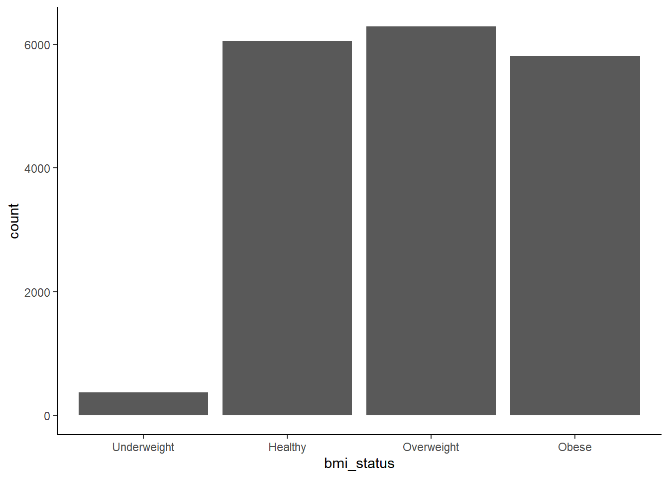
Underweight prevalence is quite low compared to the other categories, which otherwise have similar prevalence.
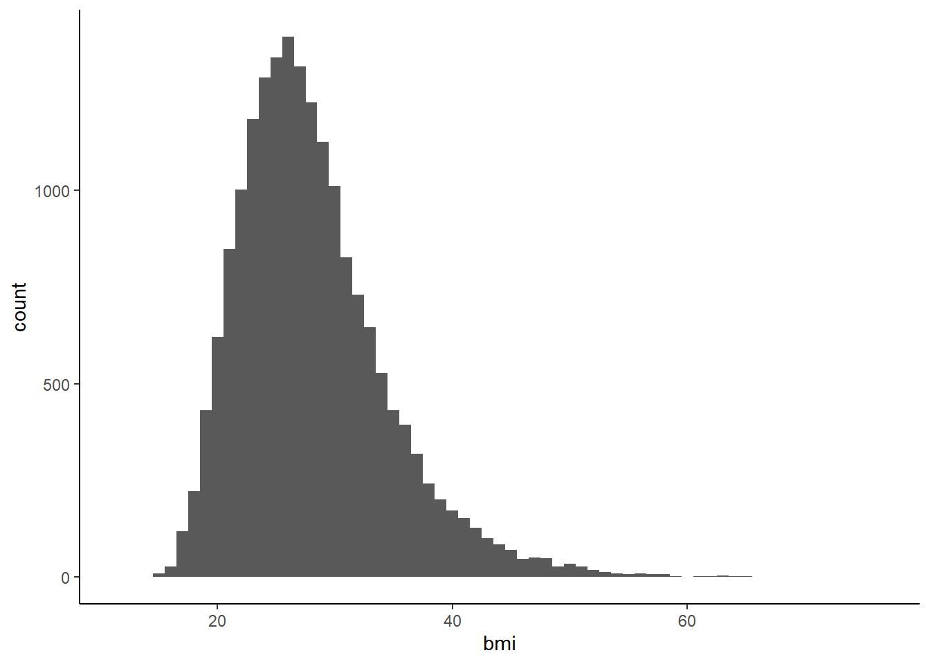
The continuous BMI distributions appears to be normal, with right skewness.
## # A tibble: 2 x 5
##   gender mean_bmi sd_bmi perc_sarc     n
##   <fct>     <dbl>  <dbl>     <dbl> <int>
## 1 female     28.6   7.10     0.200  9162
## 2 male       27.7   5.60     0.156  9374
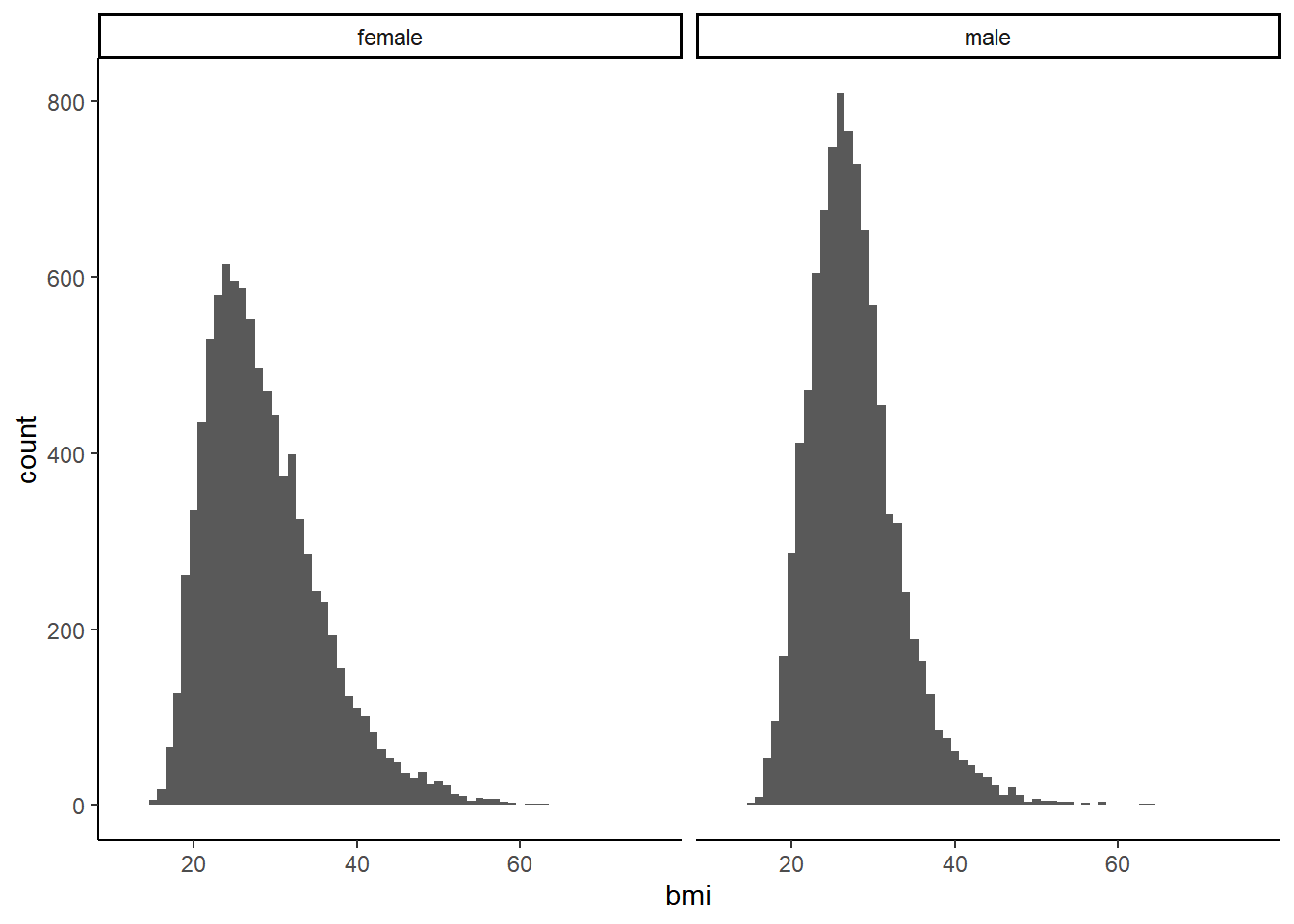
The data set is fairly evenly populated by gender. Mean BMI is quite similar between male and female as well, with a bit more variance among females. Women have a slightly higher rate of sarcopenia.
We can also check differences in BMI distribution between genders.
\(~\)
Bivariate Analysis
First we should compare total mortality prevalence stratified by different measures of body composition, since this is often the concern underlying the obesity paradox.
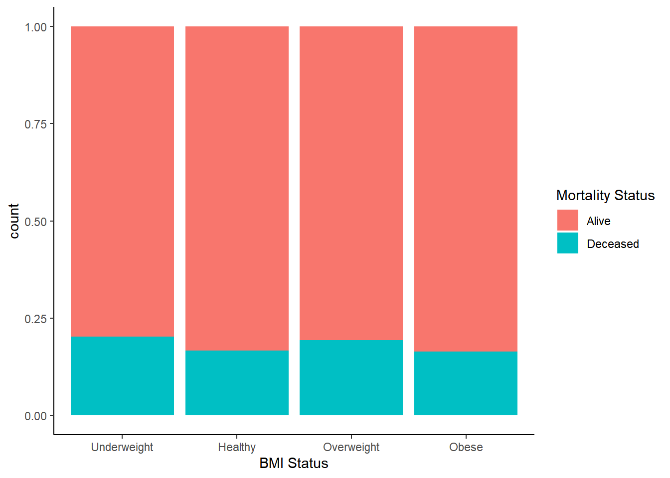
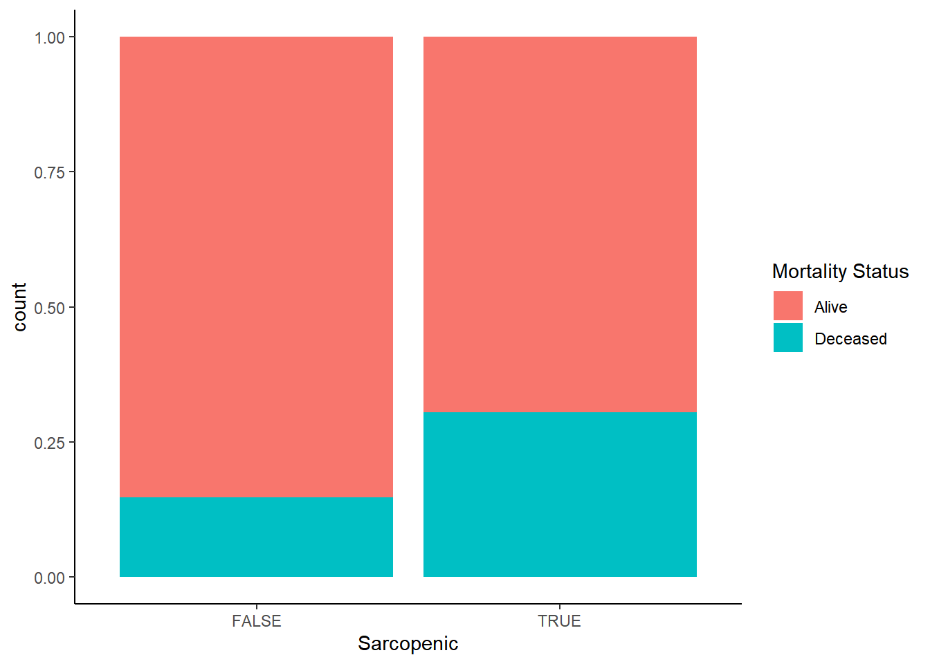
Mortality occurence does not track according to BMI status in any discernible way, but when stratifying by appendicular muscle status it’s at least twice the rate for those with sarcopenia. We have some initial indication that we might be on to something here.
Now let’s take a look at the prevalence of sarcopenia among different BMI categories.
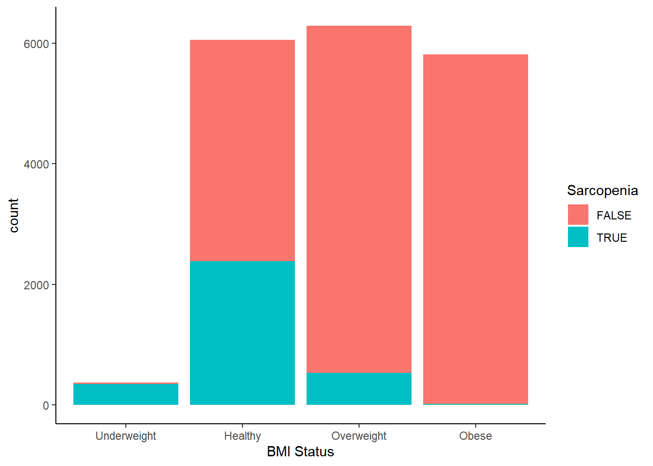
Not only is the underweight BMI category almost entirely populated by participants with sarcopenia, a substantial proportion of the healthy category is sarcopenic as well–nearly half. It seems that being given a “healthy” BMI designation has the potential to be woefully misleading. This might go some way in explaining why many investigators observe the obesity paradox in different data sets. Sarcopenia increases the risk of mortality, so if lower BMI statuses catch dramatically more sarcopenic individuals, it starts to make sense why higher BMIs sometimes appear to be protective against mortality compared to the “healthy” category. But does this mean that excess body fat is not the health risk it was thought to be, or does it mean that low muscle mass exerts a confounding effect on BMI outcomes?
At this point, we should explore how the different measures of body composition relate to each other, starting with BMI and body fat percentage.
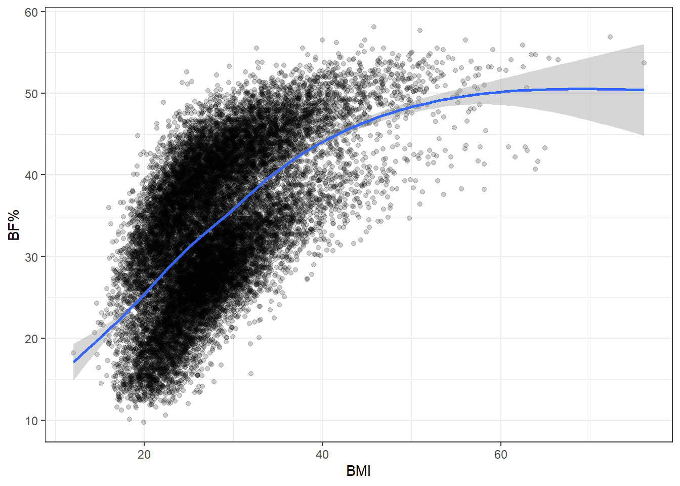
The two are pretty well associated, which is good news insofar as BMI does track body fat percentage somewhat successfully.
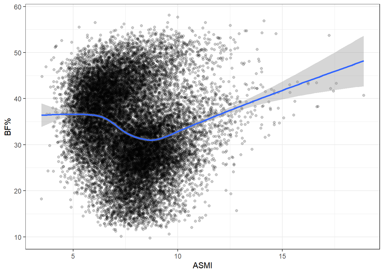
ASMI is a poor proxy for body fat. There does appear to be some clustering, though the density of points makes it hard to see clearly. The most obvious explanation for this would be gender, so let’s try stratifying by that and see if the differences match the apparent clusters above.
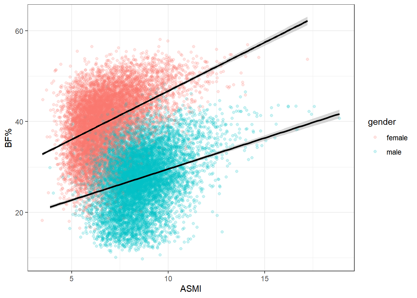
Looks like the shoe fits, as it were. We can see why running a single regression on the entirety of the data set can be misleading. Men and women tend to carry different levels of body fat and muscle, so lumping both genders together won’t provide a terribly accurate representation for analysis.
Multivariate Analysis
Let’s continue exploring various associations, starting with muscle mass and BMI. We’ll keep stratifying by gender.
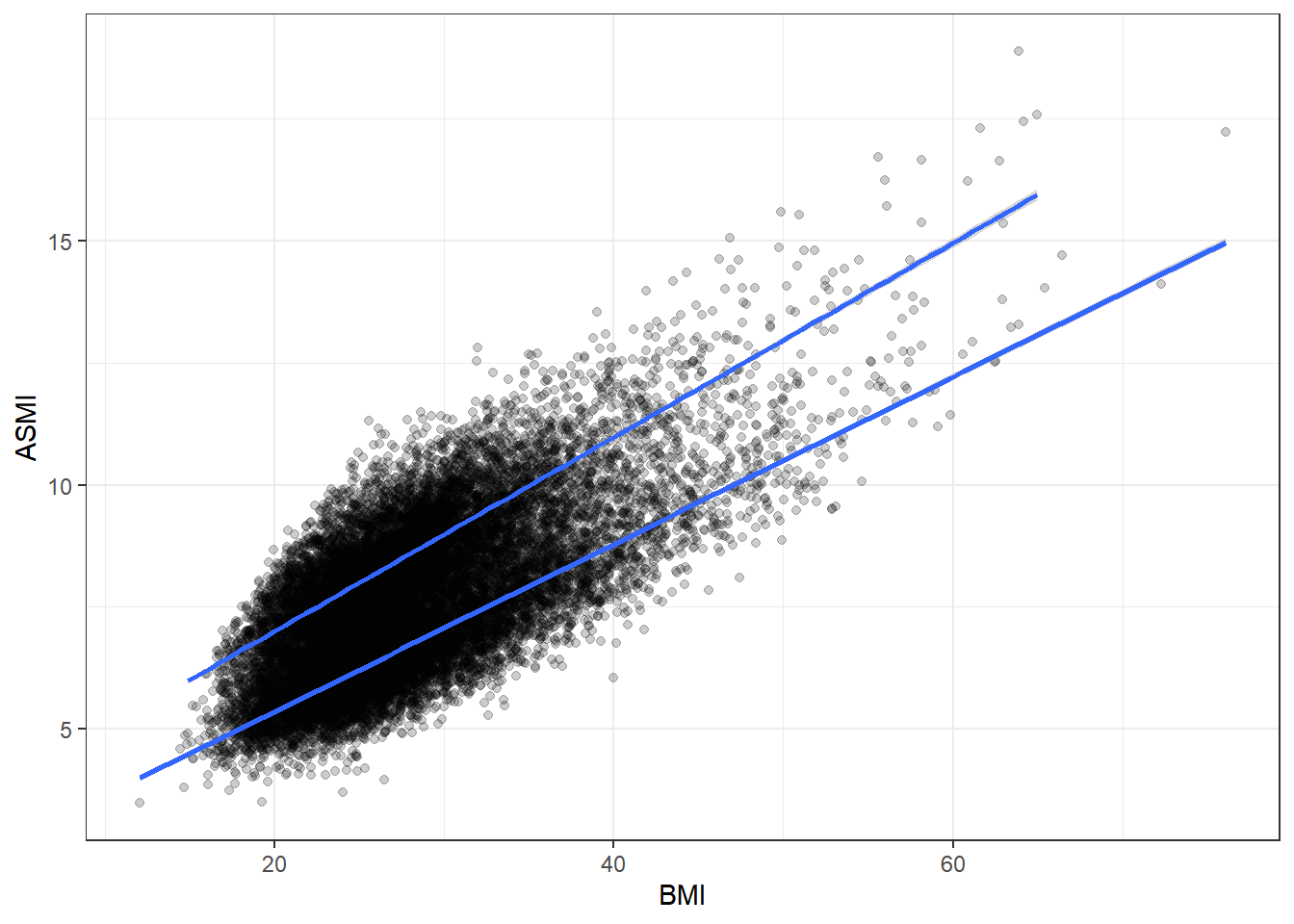
There’s a strong association here. More muscle generally corresponds to a higher BMI, which is not suprising since more muscle means more weight.
It’s important to check for any association of muscle tissue with age. Generally sarcopenia is considered an age-related disorder and a particular burdeon on the elderly. Depending on how ASMI and age are associated in the data set, our final interpretations might change.
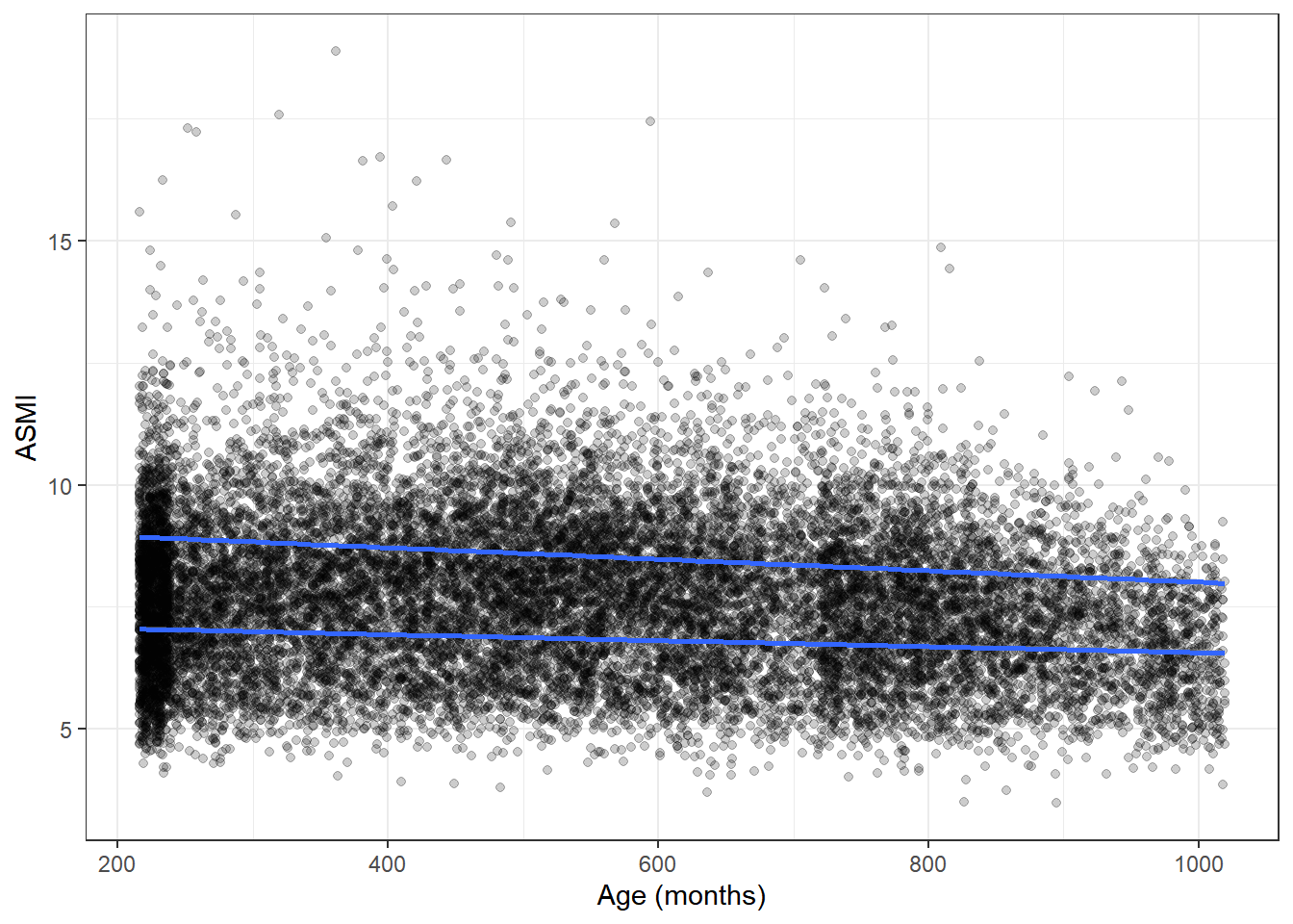
Interestingly, age and ASMI show little to no relation in the current data set, meaning that age does not appear to be a confounder for what we find with further analysis.
\(~\)
We saw that, taking all the data together, ASMI was not associated with body fat percentage. Now we’ll stratify by BMI status and see if anything changes.
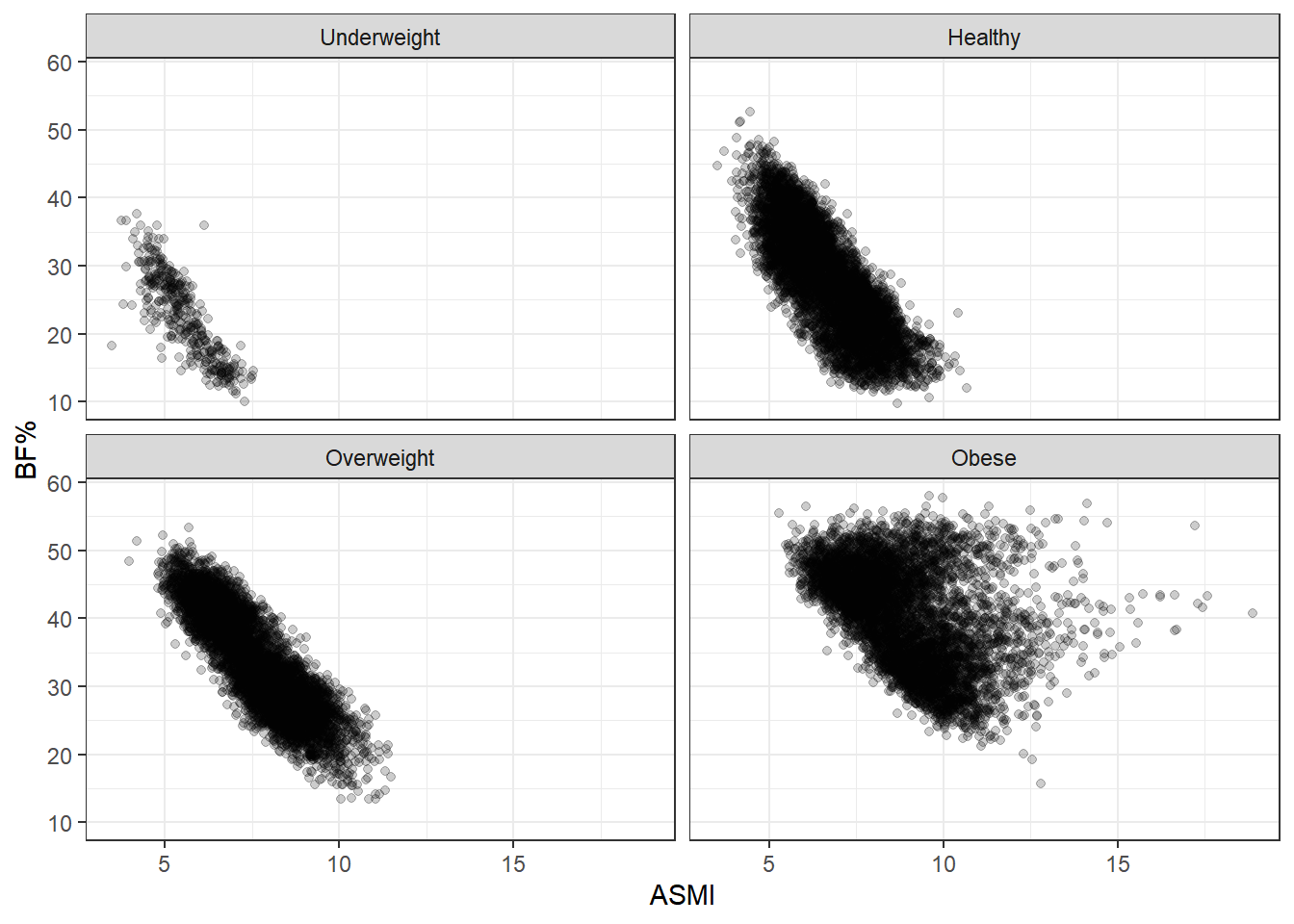
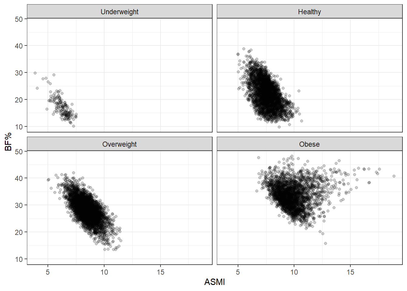
These plots are simply divisions of the body fat percentage by ASMI plot above, but splitting them better shows the range of body fat and ASMI contained in each BMI group. What stands out here is the broad range of body fat percentages included in the healthy group, from 10% to 50%, extending over almost the entire range occurring in the data set. In fact, the same can be said of the overweight group, and even to some degree of the obese group. BMI status tracks adiposity with remarkable imprecision.
Another point of note is that body fat decreases as ASMI increases. This relationship is forced by our analysis here: each plot in the grid indicates a BMI category, so as ASMI goes up, body fat must at some point go down, otherwise the observation would switch into the next BMI grouping. This is an example of collider stratification bias; controlling for BMI status introduces an artifical relationship between ASMI and body fat, so we don’t want to fool ourselves here. I think the broad ranges of BF% is the more interesting characteristic. After all, nothing about BMI says that such a range should be the case. Rather, we’d hope for a tighter spread if BMI is supposed to indicate adiposity.
To get a better idea of the range of body fat percentage within each BMI category, we can stratify by gender and compare BMI and body fat directly.
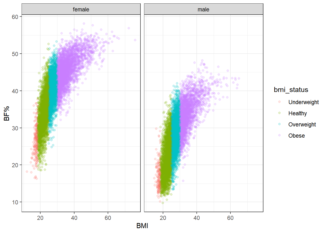
Again, there’s a remarkable spread of body fat percentage in each BMI category. Body fat increases more steeply with BMI for females than for males, but even so, the range of BF% for females is roughly 20 to 45 in the healthy category, and for males it’s roughly 12 to 35. In the overweight category the range is about 30-50% for female participants and 15-40% for male. That’s a minimum 20 percentage point spread (not counting the underweight category, which is relatively rare to begin with).
Combine this information with what we observed earlier–particularly, that nearly half of the participants with a healthy BMI score qualified as sarcopenic. It only makes sense then that body fat varies so widely at any given BMI; if so many of the participants in the healthy range are sarcopenic, then their weight has to come from somewhere, and it’s certainly not going to come from extra bone or organ tissue. Nor is it accounted for by height, since that is already included in BMI.
As a sanity check, let’s split our initial faceted plots by gender.
\(~\)
Male
Female
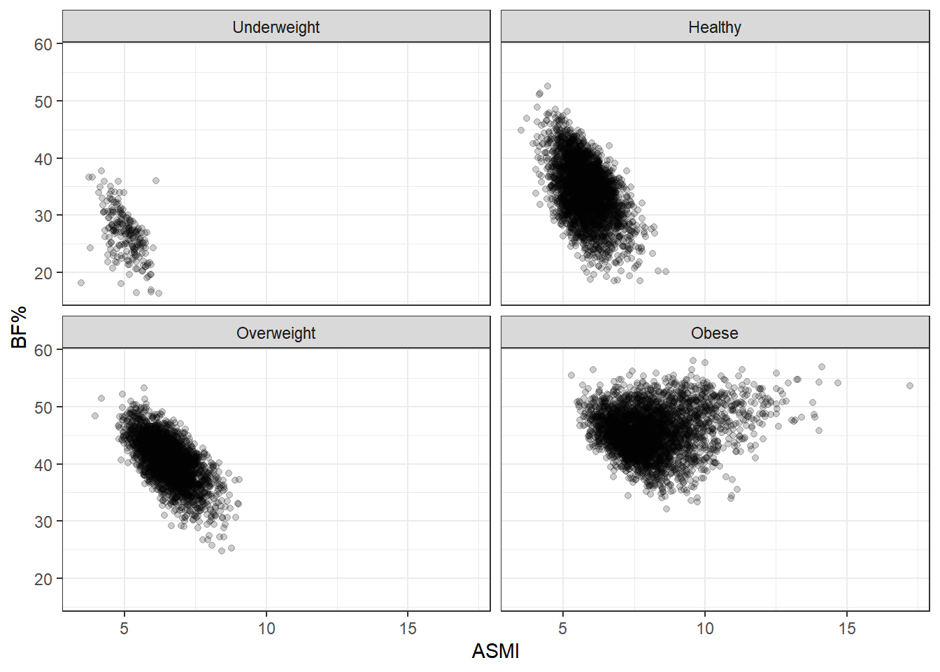
Nothing really has changed beyond the particular boundaries of the ranges. No matter what way we slice it, BMI is a rather terrible measure of body fat.
\(~\)
Let’s look at a couple more plots to get another sense of how muscle tissue status behaves in relation to BMI as a continuous variable and BF%. We’ll stratify by sarcopenia status and gender, then by sarcopenia status alone, plotting BMI against body fat percentage for both.
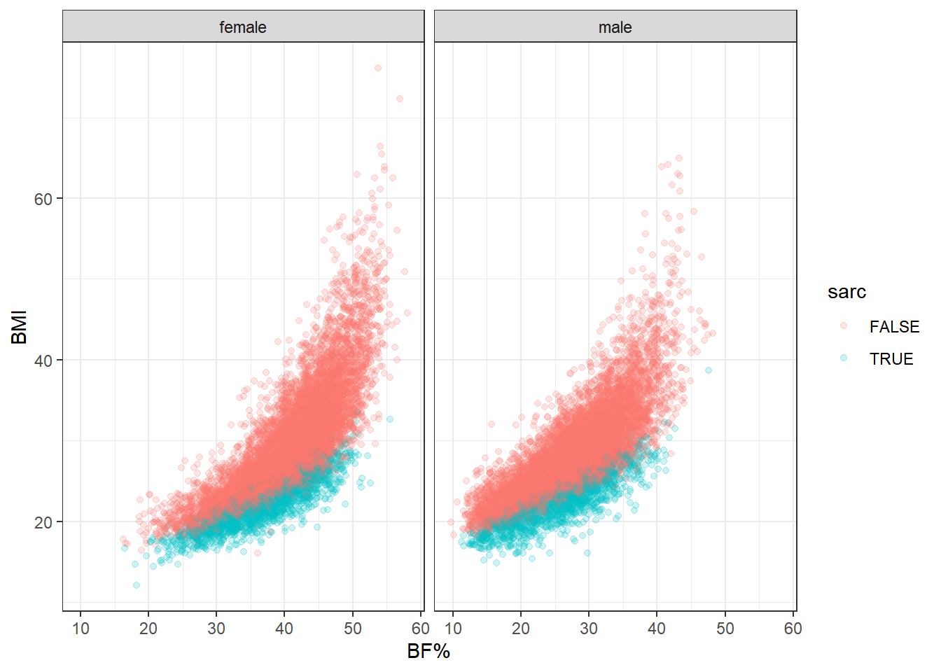
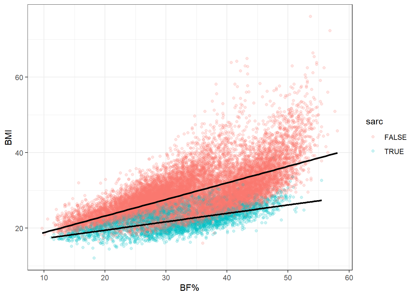
This really is the heart of the matter. At any level of body fat percentage, instances of clinically low muscle mass are gathered on the bottom end of the BMI range. And this is only a binary categorization of muscle mass. Looking again at some of the previous plots, it’s clear that ASMI ranges shift downward when moving lower on the BMI ordinal scale. It’s safe to say that low, but not clinically low, muscle mass also gathers toward the lower end of BMI within this population.
Now let’s reconsider the obesity paradox. Above-healthy BMI scores sometime correspond to equal or better mortality outcomes in ways that are counterintuitive to most practitioners and researchers considering the simultaneous association with greater prevalence of disease. But consider what we’ve seen here: an otherwise hidden determinant of health and mortality preferentially occurs at lower BMIs. In fact, it occurs in the healthy BMI category most of all.
The last point is important because the healthy BMI range is generally used as the reference category when assessing differences in mortality. Keeping in mind the observation that this category has the highest proportion of participants with low muscle mass—and I see no reason why this would not be the case in other data sets—the “paradox” starts to look more like a natural consequence of the distribution of body compostion within the BMI scale.
\(~\)
Modeling
I’ll update this section as I work on different models. One thing I’d like to do is go back to the original data and include more variables. Smoking status is an important one that can present as a confounder when modeling mortality from body composition, as smoking is associated with lower BMI but higher mortality. It might be worth including some other variables as well.
\(~\)
Conclusion
The current exploratory analysis cannot answer the question of what causes the obesity paradox, but it does provide some promising insight into potential explanations. At the very least, this analysis confirms the fact that BMI is a very low-resolution tool, and that without more precise instruments of measurement, any results concerning the association of health outcomes with obesity status warrant a surfeit of caution. The most immediate implication is that the presence of low muscle mass can mask excess fat accumulation, and if the scientific consensus about the dangers of obesity are correct, than much of that danger is being hidden in mistakenly “healthy” BMI categories.
For the same reasons, further caution should be applied to any conclusions stemming from observation of the obesity paradox itself, and the term is likely to be misleading on multiple levels. Firstly, a more appropriate name might perhaps be the “BMI dilemma,” since excess adipose tissue accumulation, as obesity is understood to be, is not limited to those higher BMI categories. Secondly, if the superior survival of BMIs above the traditionally healthy range is the consequence of preserved skeletal muscle tissue, then there simply is no paradox.
What’s most concerning is that a large majority of the population-level research into obesity and health outcomes relies on BMI to make conclusions about the role of body fat in population health. From what we’ve seen here, such conclusions are likely mistaken. The next question we’re left with is how mistaken. Furthermore, what we’ve seen here should cast doubt on how we define obesity in the first place. In terms of construct validity, BMI fails pretty miserably.
\(~\)
End
World Health Organization. (n.d.). Obesity and Overweight. who.int. https://www.who.int/dietphysicalactivity/media/en/gsfs_obesity.pdf↩︎
Centers for Disease Control and Prevention. (n.d.). Defining Adult Overweight and Obesity. cdc.gov. https://www.cdc.gov/obesity/adult/defining.html↩︎
Center for Disease Control and Prevention. (n.d.). NHANES Questionnaires, Datasets, and Related Documents. cdc.gov. https://wwwn.cdc.gov/nchs/nhanes/Default.aspx↩︎
Center for Disease Control and Prevention. (n.d.). NCHS Data Linked to NDI Mortality Files. cdc.gov. https://www.cdc.gov/nchs/data-linkage/mortality.htm↩︎
International Working Group on Sarcopenia. (May 2011). Sarcopenia: An Undiagnosed Condition in Older Adults. Current Consensus Definition: Prevalence, Etiology, and Consequences. https://www.ncbi.nlm.nih.gov/pmc/articles/PMC3377163/↩︎